Plotly Library

By David Do
December 2nd, 2024 | 8 min read

Introduction to Plotly: A Powerful Tool for Interactive Data Visualization

In today's data-driven world, the ability to visualize complex datasets clearly and interactively is essential. Plotly is one such tool that has gained widespread popularity for its versatility and ease of use in creating interactive and publication-quality visualizations. In this blog post, we'll introduce you to Plotly, explore its basic features, and show you why it is a useful data visualization toolkit.

What is Plotly?

An open-source graphing library that allows you to create interactive, web-based graphs and dashboards with minimal effort
Supports a wide range of chart types, including line plots, scatter plots, bar charts, heatmaps, 3D surface plots, etc.
Ease of integration with Python, R, and JavaScript

Why choose Plotly?

Interactivity: Plotly visualizations are inherently interactive, allowing users to zoom, pan, hover, and click on data points to explore the underlying data more deeply
Ease of Use: Users can customize almost every aspect of their charts, from colors and fonts to annotations and hover effects, ensuring that the visualizations align with the desired brand or style
Compatibility: Plotly provides libraries that work seamlessly in each environment, whether users are working in Python, R, or JavaScript

Getting Started with Plotly in Python

Installation

You can install Plotly using pip:

pip install plotly

Let’s create a simple line plot to illustrate the basics. We will use Plotly Express, a high-level interface to Plotly, which makes it easy to create complex plots with just a few lines of code.

import plotly.express as px

# Sample data
data = {
    'Year': [2015, 2016, 2017, 2018, 2019, 2020],
    'Sales': [200, 220, 230, 250, 270, 300]
}
# Create a line plot
fig = px.line
(data, x='Year', y='Sales', title='Yearly Sales Growth')

# Show the plot
fig.show()
# Create a line plot
fig = px.line
(data, x='Year', y='Sales', title='Yearly Sales Growth')

# Show the plot
fig.show()

We can create a simple interactive line plot like this that we can zoom, pan, and hover over to see the details.

Plotly Examples in RAP®

1. Query & Plot Originations broken out by Runoff Type (aggregate) from a Runoff Portfolio

query = """
select
    substring(origination_date,1,6) as Origination_Date,
    Estimated_Payoff_Type,
    count(*) as Cnt,
    format_number(sum(loan_amount),0) as Original_Balance
from {}.runoff_results{}
where substring(origination_date,1,4) >= 2015
group by
    substring(origination_date,1,6),

For Plotly visuals to render within RAP, we must convert the above spark data frame into pandas data frame, and plot each visual in its own local mode (%%local).

# Convert spark df to pandas df
%%spark -o query

# Plotly - Originations broken out by Runoff Type
%%local
from plotly.offline import plot, init_notebook_mode
init_notebook_mode(connected = True)
import plotly.graph_objs as go

query_agg = query.groupby(['Origination_Date', 'Estimated_Payoff_Type'])[['Cnt']].sum().unstack().fillna(0)

fig = go.Figure(
    data = [
        go.Bar(name="N/A", x=query_agg.index, y=query_agg["Cnt"]["N/A"]),
        go.Bar(name="Deed Transfer", x=query_agg.index, y=query_agg["Cnt"]["Deed Transfer"]),
        go.Bar(name="New Mortgage", x=query_agg.index, y=query_agg["Cnt"]["New Mortgage"]),
    ]
)

layout = go.Layout
(title="Originations broken out by Runoff Type", title_x=0.5, width=1200, height=1000, xaxis=dict
(type="category", dtick=1, fixedrange=True, tickangle=45), plot_bgcolor="black", legend={'title': {'text': 'Runoff Type'}})

fig.update_layout(xaxis_title="Origination Date", yaxis_title="Count", barmode="stack")
plot(fig)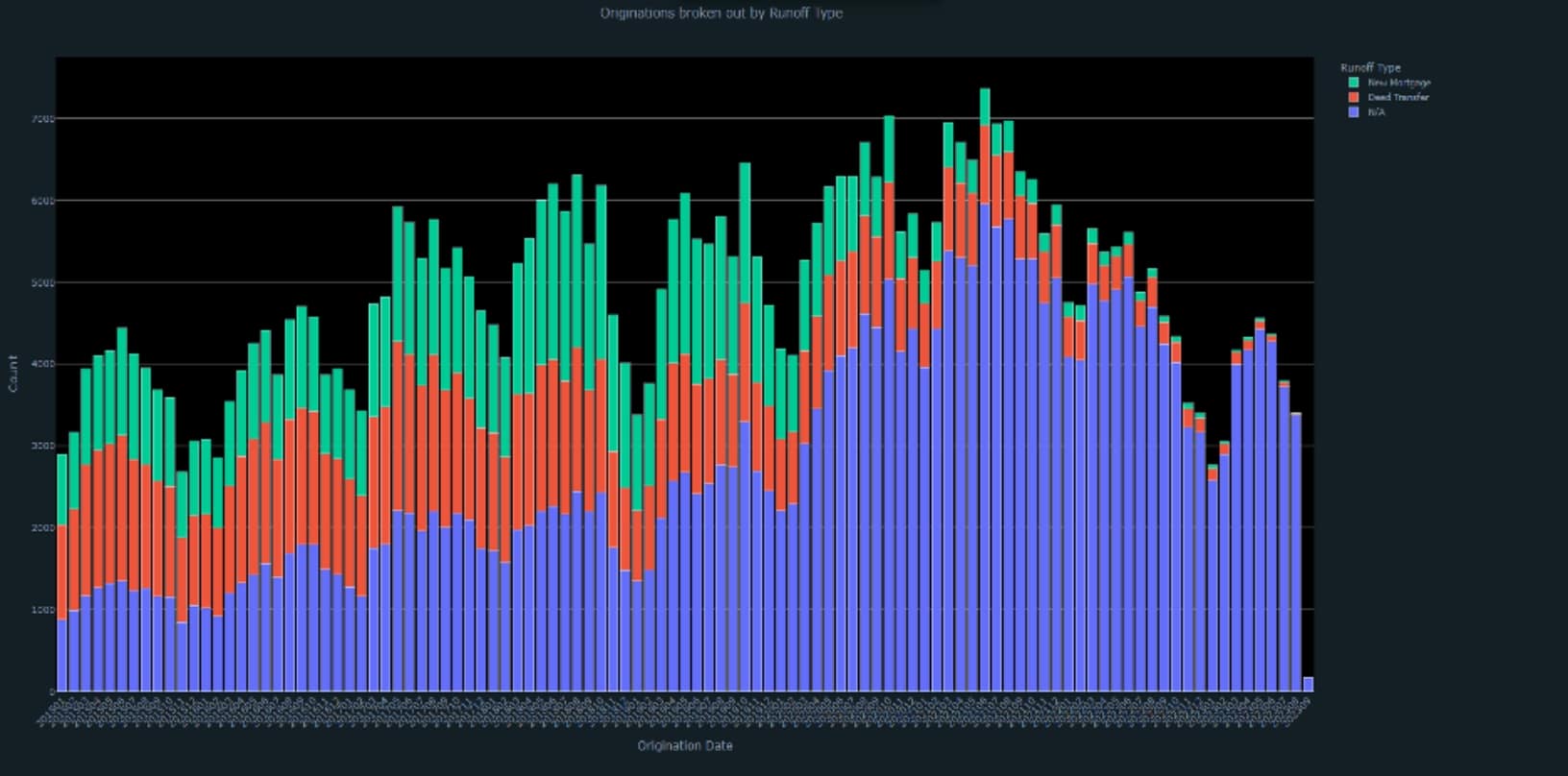

2. Query & Plot Runoff by Type

query = """
select
    substring(Next_Transaction_Date,1,6)
 as Next_Transaction_Date,
    Estimated_Payoff_Type,
    count(*) as Cnt,
    format_number(sum(loan_amount),0)
 as Original_Balance
from {}.runoff_results{}
where Next_Transaction_Date >= 20150101
group by
    substring(Next_Transaction_Date,1,6),
    Estimated_Payoff_Type
""".format(db_to_use, lender_table_extension)

query = spark.sql(query)

# Convert spark df to pandas df
%%spark -o query

# Plotly - Runoff by Type
%%local
from plotly.offline import plot, init_notebook_mode
init_notebook_mode(connected = True)
import plotly.graph_objs as go

query_agg = query.groupby(['Next_Transaction_Date', 'Estimated_Payoff_Type'])[['Cnt']].sum().unstack().fillna(0)

fig = go.Figure(
    data = [
        go.Bar(name="Deed Transfer", x=list(query_agg.index.values), y=query_agg["Cnt"]["Deed Transfer"].values),
        go.Bar(name="New Mortgage", x=list(query_agg.index.values), y=query_agg["Cnt"]["New Mortgage"].values),
    ]
)
layout = go.Layout(title="Runoff by Type", title_x=0.5, width=1200, height=1000, xaxis=dict
(type="category", dtick=1, fixedrange=True, tickangle=45),
 plot_bgcolor="black", legend={'title': {'text': 'Runoff Type'}})

fig.update_layout(xaxis_title="Next Transaction Date", yaxis_title="Count", barmode="stack")
plot(fig)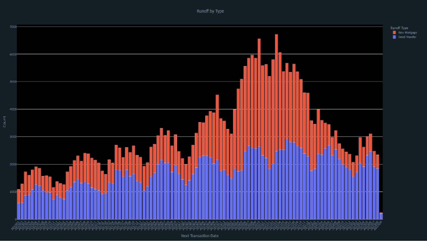

3. Query & Plot Runoff - Lender Competition

1) Create Runoff Lender Aggregation View

query = """
create or replace temp view runoff_results_lender_aggregation{} as

select
    row_number() over (partition by substring(Next_Transaction_Date,1,4) order by count(*) desc) as instance,
    substring(Next_Transaction_Date,1,4) as Next_Transaction_Date,
    g.Next_Transaction_lender_name_clean,
    count(*) as Cnt
from {}.runoff_results{} r
where Estimated_Payoff_Type = 'New Mortgage'
    and Next_Transaction_Date >= 20150101
    and Next_Transaction_Recapture = 'Lost'
    --and r.Next_Transaction_lender_name not like '{}'
    --and r.Next_Transaction_lender_name not like '{}'

group by
    substring(Next_Transaction_Date,1,4),
    g.Next_Transaction_lender_name_clean
order by
    substring(Next_Transaction_Date,1,4), Cnt desc
""".format(lender_table_extension, db_to_use, lender_table_extension, lender_name_search, lender_name_search_2)

query = spark.sql(query)

2) Query Lender Competition

query = """

select
    Next_Transaction_Date,
    case when instance <= 5 then Next_Transaction_lender_name_clean else 'a) Other' end as Next_Transaction_lender_name_clean,
    sum(Cnt) as Cnt
from runoff_results_lender_aggregation{}
group by
    Next_Transaction_Date,
    case when instance <= 5 then Next_Transaction_lender_name_clean else 'a) Other' end
""".format(lender_table_extension)

query = spark.sql(query)

3) Visualize lender competition in stacked bar chart

# Convert spark df to pandas df
%%spark -o query

# Plotly - Runoff - Lender Competition
%%local
from plotly.offline import plot, init_notebook_mode
init_notebook_mode(connected = True)
import plotly.graph_objs as go
import plotly.express as px
fig_data = []
fig_layout = {}

query_agg = query.groupby(['Next_Transaction_Date', 'Next_Transaction_lender_name_clean'])[['Cnt']].sum().unstack().fillna(0)

period = query_agg.index
lenders = query_agg.columns.tolist()
data = []

for i in range(len(period)):
    for j in range(len(lenders)):
        label = lenders[j]
        data.append(go.Bar(x=[str(period[i])[:4]], y=[query_agg[lenders[j]][i]], name=label))

fig = go.Figure(
    data = data,
    layout = go.Layout(
        title="Runoff - Lender Competition",
        title_x=0.5,
        width=1200,
        height=1000,
        xaxis=dict(type="category", dtick=1, fixedrange=True, tickangle=45),
        plot_bgcolor="black",
        legend={'title': {'text': 'Lender'}}
    )
)

fig.update_layout(
    xaxis_title="Next Transaction Date",
    yaxis_title="Count",
    barmode="stack",
    showlegend=True,
    legend_itemclick="toggleothers",
    legend_itemdoubleclick="toggle",
    legend_traceorder="normal",
    legend_orientation="h",
    legend_title="Lender"
)

plot(fig)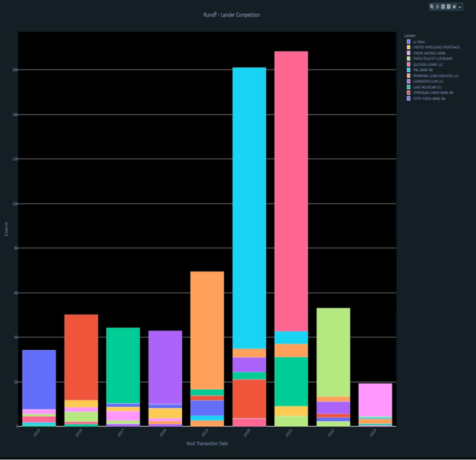

David Do, Data Scientist

David has 3 years of experience as a data scientist, specializing in financial services and technology, with a focus on building ML predictive models and implementing data-intensive client-side solutions. He holds a Bachelor of Science in Data Science from UC San Diego and is currently pursuing a Master of Science & Engineering in Data Science from the University of Pennsylvania. David brings solid hands-on expertise in advanced analytics in the mortgage technology space.